Table of contents
Open Table of contents
New Features
- 3D renderings of Lunar Rover traverses using LRO data courtesy of NASA Goddard Space Flight Centre
- Mission dashboard at-a-glance
- Transcript and commentary search
- Hours of additional rare footage courtesy of archive producer, Stephen Slater
- Hundreds of transcript and timing corrections
Recreating the Moon – Lunar Reconnaissance Orbiter
This spring, after the wonderful attention died down from the release of the site last December, I came across some incredible data pertaining to the Apollo landing sites that was recently published by the LRO mission team.
The data includes very high-resolution photography and topology data of the valley of Taurus-Littrow, where Apollo 17 landed 44 years ago today.
I realized that I could use this data to recreate the landing area in 3D and possibly simulate some of the segments of the Apollo 17 mission that did not include television transmissions.
During the three-day stay on the lunar surface, the remotely controlled TV camera only transmitted a signal when the Lunar Roving Vehicle (LRV) was stationary (the camera and transmission antenna were both attached to the LRV).
When they drove from place to place on the lunar surface (they traveled a total distance of 35.9 km), the high-gain television antenna needed for the video transmission was bouncing around too much to attempt to maintain a transmission to Earth.
Because of this, only audio transmissions are available for much of the crew’s time working on the surface.
I contacted Dr. Noah Petro, Deputy Project Scientist of the LRO mission at Goddard, and asked for his assistance in understanding the data available online.
Dr. Petro and his colleagues very generously provided me with even higher resolution data and photography and were hugely helpful in helping me to better understand how to work with it.
I pulled this data into Cinema4D, a piece of professional 3D rendering software, to see if I could create a workable simulation of being in close proximity with the Apollo 17 astronauts as they drove around on the surface.
 High-resolution topology data of the Taurus Littrow valley
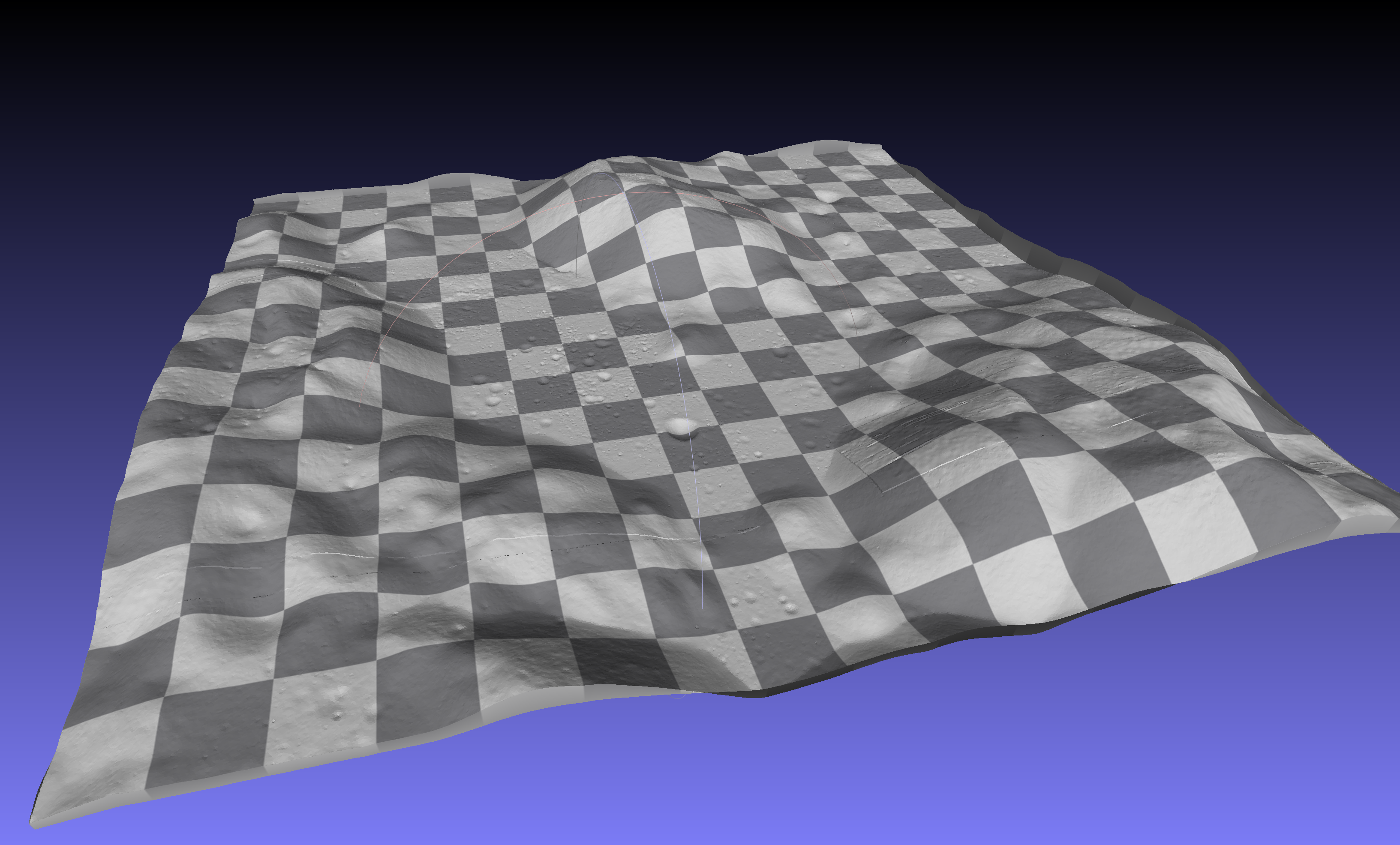 Test displacement mesh using topology data
The first step was to displace a 3D mesh using the LRO topology data.
This, in theory, would recreate the texture of the lunar surface, down to individual craters.
The image above shows one of my first tests.
You can see the valley floor and, if you know where to look, the landing site of the Lunar Module.
I was on to something.
The topography data provided to me by Noah and his team is at 16-bit resolution—this means that the height of each point on the ground is represented with extreme precision.
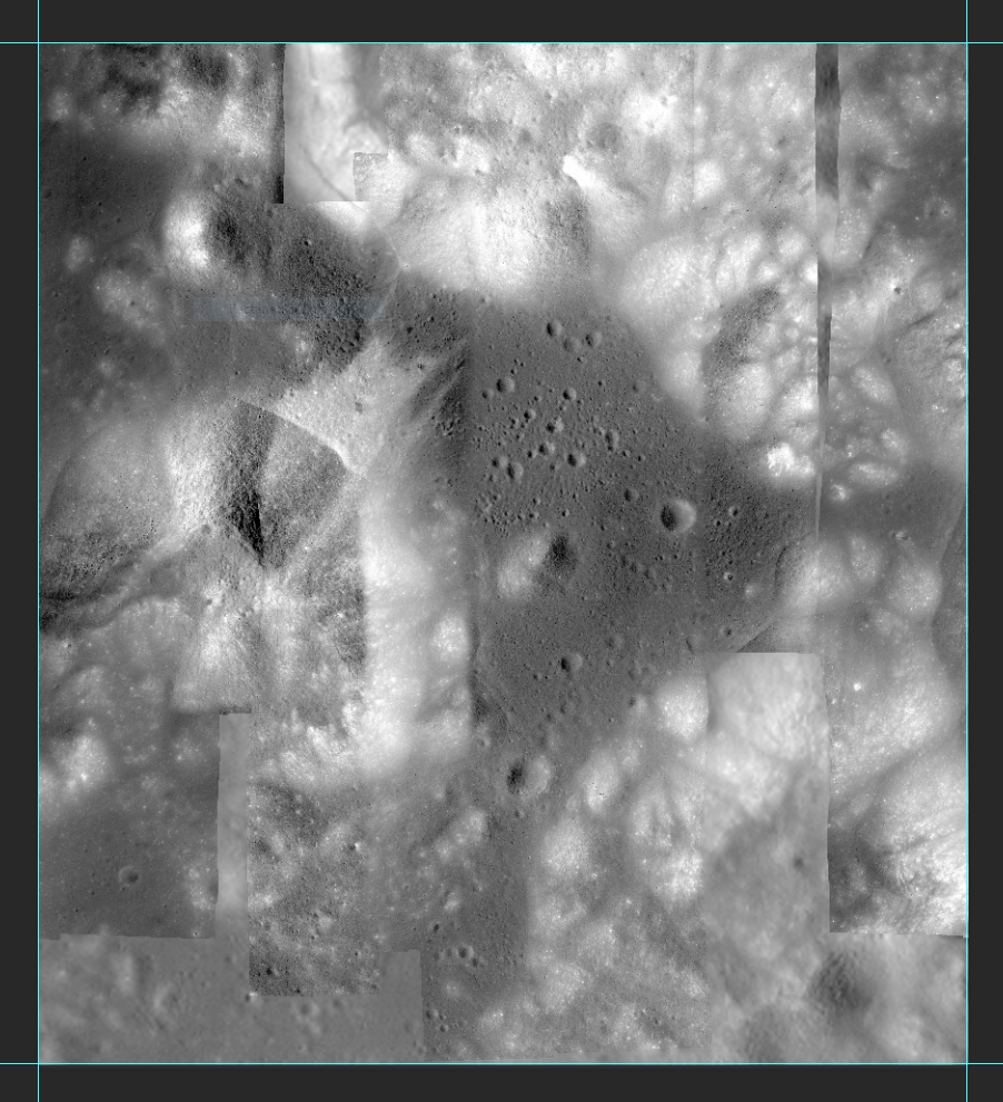 High-resolution photography of the Taurus Littrow valley
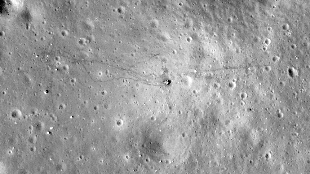 Close-up of Apollo 17 landing area
The next step was to texture the surface using the high-resolution photography taken by the LRO.
This would have the added benefit of including real sun shading from the lunar surface contained in the photos themselves.
I wouldn’t have to artificially light the artificial 3D scene at all.
The images captured by the LRO are in such high resolution that you can see the lander and even the footprints left behind by the crews of all of the Apollo missions.
The close-up image above shows the Apollo 17 landing site.
Note the footprints running east and west from the lander.
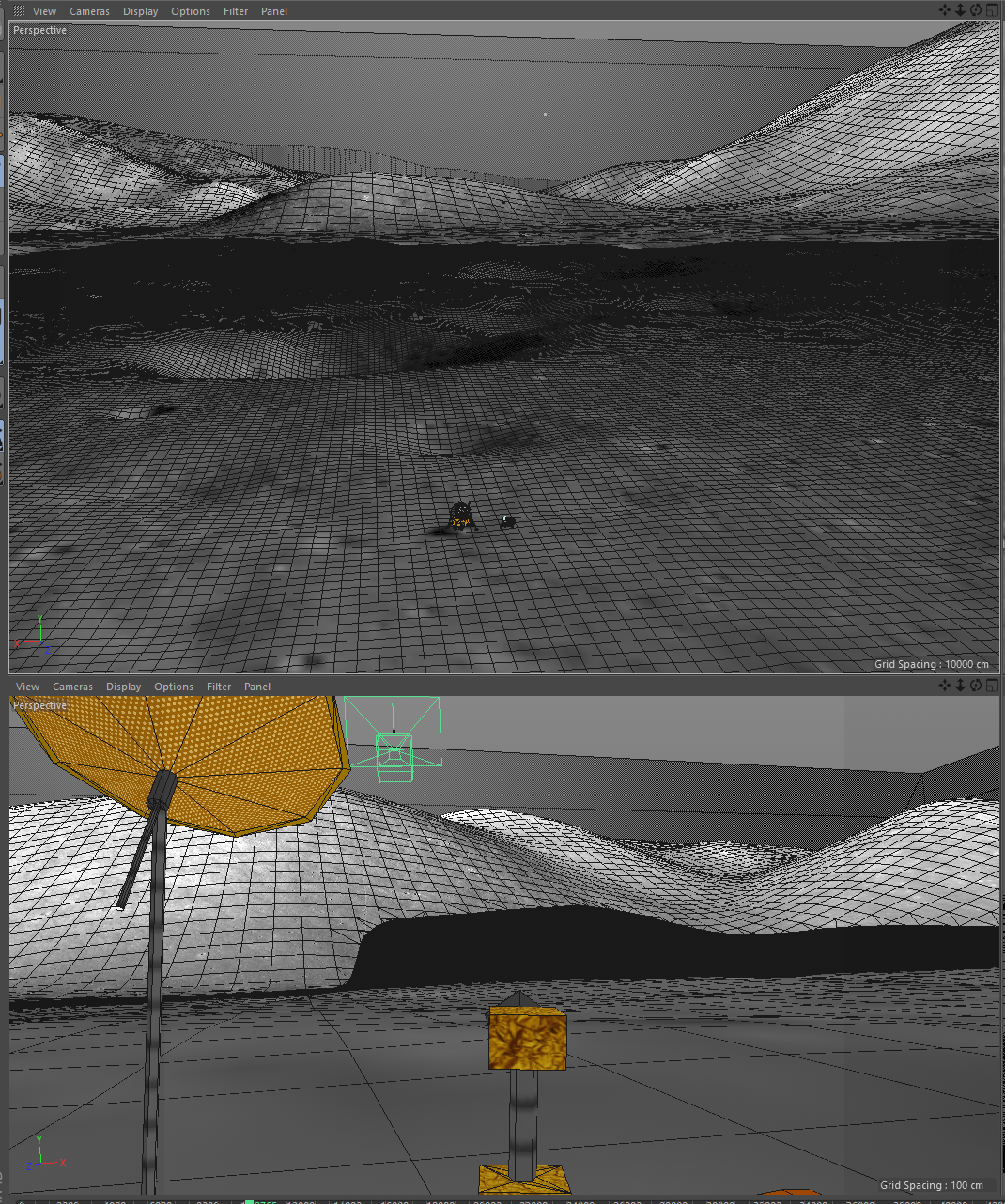 Top: textured surface mesh previsualization; Bottom: view from the Lunar Rover previsualization
The result of combining the displaced mesh with the photography is a textured mesh that is a replica of the real lunar surface to an accuracy of approximately 60 cm per pixel.
The dataset is so large (and therefore so accurate) that it requires 64 GB of RAM to open the texture file alone.
In the image above, you can see the terrain mesh textured with the lunar photography.
Here I’m showing the surface mesh lines to illustrate how the data works together to create a realistic reconstruction of the lunar surface.
In the photo, you can also see small models of the Lunar Module and the LRV.
I found these models online and scaled them appropriately to the image data.
In fact, I used the actual tracks on the lunar surface left by the real LRV to verify that I got the scale right!
Incredible.
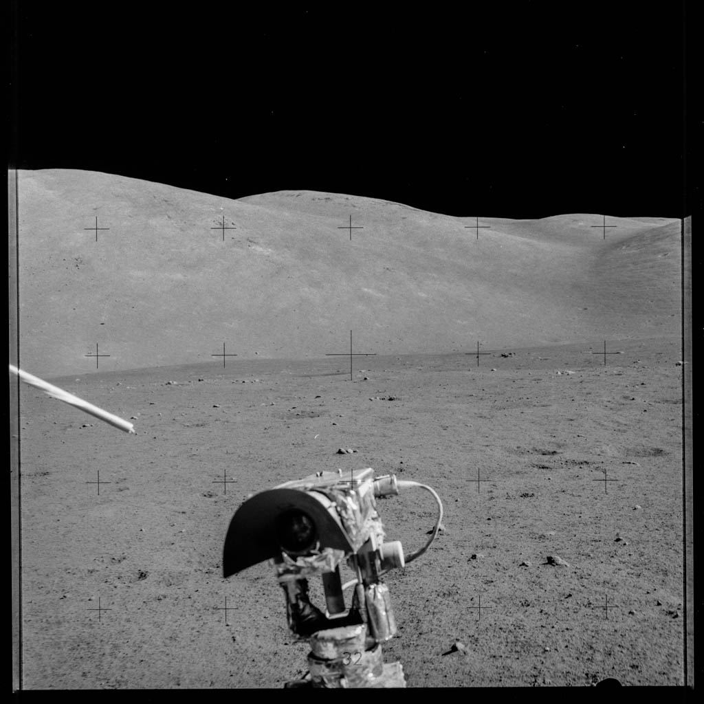 Actual photo taken by the crew of the same view as the 3D model above
To test the accuracy of the result, I placed a virtual camera in 3D space into the LRV at the approximate position of Jack Schmitt’s Hasselblad camera.
Schmitt was tasked with taking LRV traverse photos as they drove around on the Moon.
Each of these photos has the TV camera that was mounted at the front of the LRV at the bottom center of the frame.
For this test, I pointed the LRV northeast from the landing site and compared the virtual 3D “photo” with a real mission photo.
You can see the same hills in the background at roughly the same scale.
The lighting is different, but that’s because the LRO scanned the area at a time of lunar day that was different than when they visited the valley in 1972.
Follow the Path
 Apollo 17 Traverse Map
The next step was to understand, in detail, where exactly the crew traveled on the lunar surface. Using original post-mission analysis documents from the 70s (left), I roughly plotted out the path followed from station to station. This wasn’t detailed enough to account for every small deviation and turn made by Cernan as he drove. To reach the next level of granular detail, I “timed” out the traverses using the transcript and audio recordings I had restored for apollo17.org previously.
Here is an example of a timing transcript. This is the first traverse from around the Lunar Module to Station 1.
Here is an example of a timing transcript. This is the first traverse from around the Lunar Module to Station 1.
ALSEP to Station 1
0:00:00 - 121:36:14 - TV off
0:07:29 - 121:43:43 - LRV starts moving first turns northwest a bit, then east
0:08:32 - 121:44:46 - avoiding a crater
0:09:29 - 121:45:43 - LRV at LM
0:09:45 - 121:45:59 - LRV starts moving to SEP site
0:11:10 - 121:47:24 - Stopped at SEP bearing 278, 003
0:14:48 - 121:51:02 - On the move to Station 1, turning to 181
0:15:27 - 121:51:41 - Trident east
0:16:07 - 121:52:21 - "whoa, watch it" (falling in crater)
0:16:26 - 121:52:40 - "you've got another hole on your right here"
0:16:33 - 121:52:47 - "why don't you go left there"
0:17:03 - 121:53:17 - "we need to head south"
0:17:31 - 121:53:45 - headed due south
0:18:00 - 121:54:14 - abreast of, or just above Trident crater
0:18:00 - 121:54:14 - 330, 0.3
0:19:48 - 121:56:02 - turning to 181 degrees
0:22:28 - 121:58:42 - 0.7km from steno
0:23:24 - 121:59:38 - abreast of Powell
0:23:56 - 122:00:10 - 342, 0.9
0:24:57 - 122:01:11 - Steno at 9 o'clock
0:26:47 - 122:03:01 - 346, 1.1
0:27:48 - 122:04:02 - Parked at 180
0:30:35 - 122:06:49 - TV on
This shows that a 30 minute, 35 second video is required and includes all of the movements mentioned by the crew during the traverse. Using this as the basis for a 3D animation, I plotted timing of the LRV’s movement according to this using the 70s mapped course as the basis. This first round of timed movement would show the rover moving at a constant rate from timed event to timed event. The speed of the LRV’s movement is known to have averaged 13 km/h (max 18km/h going down hill). I could error check the timed course animation I created from the raw data by making sure it corroborated the LRV’s actual historical speed. Many errors in course were caught this way and corrected. Further, the photography taken by Schmitt on each traverse could be directly compared to the animated orientation of the rover as the traverse progressed. These snapshots captured not only terrain in front of the rover, but also the orientation of the rover on the surface. Having timed these photos last year, I could use them as a basis for understanding how the LRV zigged and zagged across the surface from station to station.
Rendering the Moon
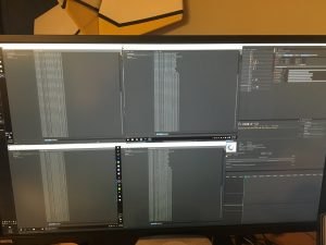 Rendering the Moon
Rendering 3D animation is very computer-intensive work—especially an animation with such high-resolution textures and meshes. Cinema 4D has a great feature: the ability to distribute the workload across machines. I borrowed as many computers as I could muster from friends and colleagues. These ranged in capability and age, but every little bit of CPU resources helped. With this makeshift render farm, I heated my basement for about 6 weeks this summer rendering out the animations of each traverse—14 in all.
The resulting animations far exceeded my expectations. The last step was to drop them into the video projects I had used to originally reconstruct the transcripts and re-export them to YouTube.
Here are links to the LRO animated LRV traverses for those interested:
- http://apollo17.org?t=119:04:49 - Rover driving to Apollo Lunar Surface Experiments Package (ALSEP) site
- http://apollo17.org?t=121:36:13 - Rover driving to Station 1 (Steno Crater)
- http://apollo17.org?t=122:35:47 - Rover driving from Station 1 to SEP site to end EVA1
- http://apollo17.org?t=141:30:47 - Rover driving to Station 2 (South Massif - Nansen Crater)
- http://apollo17.org?t=143:45:51 - Rover driving to Station 3 (Lara Crater)
- http://apollo17.org?t=145:03:55 - Rover driving to Station 4 (Shorty Crater)
- http://apollo17.org?t=145:54:47 - Rover driving to Station 5 (Camelot Crater)
- http://apollo17.org?t=146:52:35 - Rover driving to from Station 5 back to Lunar Module to end EVA2
- http://apollo17.org?t=164:21:27 - Rover driving to Station 6 (Tracy’s Rock)
- http://apollo17.org?t=166:02:10 - Rover driving to Station 7 (North Massif)
- http://apollo17.org?t=167:32:28 - Rover driving to Station 8 (Sculptured Hills)
- http://apollo17.org?t=167:32:28 - Rover driving to Station 9 (Van Serg Crater)
- http://apollo17.org?t=168:47:07 - Rover driving back to Lunar Module to end EVA3
- http://apollo17.org?t=169:52:48 - Cernan driving rover to its final resting place
Comments
-
Apollo16uvc (March 23, 2017 at 3:39 pm):
This is one of the greatest websites ever made on Apollo.
Thank you so much for your effort, I can’t thank you enough.
Where did you get all the Apollo 17 Television footage? I’d love to look through the archive on my own accord.- Feist (March 23, 2017 at 5:29 pm):
Thanks, I’m really glad you’re liking it!
The TV footage is part of the NASA archives. Sadly, it’s not readily available in its totality. However, Spacecraft Film released a set of DVDs a little over a decade ago that includes most of it. Spacecraft Films
- Feist (March 23, 2017 at 5:29 pm):
-
Nick Devereux (May 28, 2017 at 5:29 pm):
Amazing!
Well done and thank you. Apollo17.org is an amazing accomplishment.
I have no idea why the NASA Public Affairs Office is unable to do as good a job chronicling human spaceflight as you have done here for Apollo 17. Having everything collected in one place in chronological order makes it so much easier to comprehend.
Do you plan to similarly archive other missions? I hope so.- Feist (May 29, 2017 at 8:51 am):
I’m glad you like the site. Don’t be too hard on NASA PAO and the NASA History Office. They do a ton of great work. NASA isn’t a museum and is focused on future missions.
Other missions are a possibility. Possibly Apollo 11 next given that the 50th anniversary is in 2019. We’ll see.
- Feist (May 29, 2017 at 8:51 am):
-
jeff thomson (June 24, 2017 at 3:27 am):
64 GB is required for opening a single file in that kind of large animated video production. The resources used for rendering are really big. -
Mac Bryan (June 24, 2017 at 3:34 am):
Making a 3D animation video as realistic as possible just through textures is tough, but you have done it greatly. -
Gabriel Frank (November 9, 2017 at 1:41 am):
Hi Ben!
This is an incredible and inspiring project. I especially appreciate the in-flight and early mission sequences since they aren’t available anymore on Apollo Lunar Surface Journal.
Thanks for doing all this!- Feist (November 9, 2017 at 9:29 am):
Thank you very much for the kind note. The companion site to the Apollo Lunar Surface Journal is the Apollo Flight Journal. I’ve been working with David, the author of the Flight Journal, to get my Apollo 17 content online in that more traditional format. Apollo Flight Journal
- Feist (November 9, 2017 at 9:29 am):
-
Michael Williams (November 9, 2017 at 8:05 pm):
Hi Ben,
Thank you for the great project, I’ve been enjoying it immensely.
I’ve been trying to catch the realtime “In-Progress” feed right at the beginning. Would there be a way to calculate when it would restart each time?- Feist (November 10, 2017 at 9:00 am):
The simulation starts at exactly 9:55:39 pm EST on the 6th of each month. If you wait until Dec 6th this year, you’ll be watching the mission exactly 45 years later, to the second.
- Feist (November 10, 2017 at 9:00 am):
-
John Eric Thompson (November 15, 2017 at 11:45 am):
I LOVE this site!!!
Great work and well done. -
Jordan L (December 10, 2017 at 3:57 am):
WOW! Thank you so much for providing such a unique way to experience history. I may have to download Orbiter and NASSP again and get that synced on a second monitor. It will no longer be unnaturally quiet! -
Jørgen F. Bak (December 12, 2017 at 12:43 pm):
Amazing site – I really enjoy it.
However, the sound file seems to be missing from 128:47 to 136:27 – I’m trying to live through the endeavor. But there is a hole in the sound tapestry.- Feist (December 13, 2017 at 3:03 pm):
Not all of the recordings have been digitized. I have to wait patiently for NASA to get to the missing segments.
- Feist (December 13, 2017 at 3:03 pm):
-
Otha H Vaughan Jr (December 14, 2017 at 5:45 pm):
Ben: I am an MSFC Retired Engineer who developed the Lunar Surface Design Criteria for the Lunar Rover. Also helped in creating our lunar driving simulator. -
Jhonny (December 19, 2017 at 3:23 pm):
Somewhere there seems to be an error in mission time. The official mission time is 12d, 13h, 51m and 59s, equating to a mission timer at splashdown of 301:51:59, but it actually was 504:31:50.- Feist (December 19, 2017 at 5:14 pm):
This time discrepancy is due to the launch delay. You can read about it here: Changing the Clocks
- Feist (December 19, 2017 at 5:14 pm):
-
Tim Chambers (December 31, 2017 at 2:16 pm):
How do you submit corrections? I am seeing a number of discrepancies between voice and transcript.- Feist (January 24, 2018 at 7:48 pm):
Please feel free to email me at [email protected].
- Feist (January 24, 2018 at 7:48 pm):
-
Mike Smithwick (July 15, 2018 at 5:05 pm):
Amazing site Ben! I have a little information you might want to add: I have the flown copy of the “CSM Updates” manual from Apollo 17. It has notes for every SPS burn. I can send you images of the pages if desired.- Feist (July 17, 2018 at 3:00 pm):
Thanks Mike. A flown copy of the CSM updates is pretty cool indeed. So you have the pad notes taken down by the crew during readings?
- Feist (July 17, 2018 at 3:00 pm):
-
David (October 21, 2018 at 6:08 pm):
This. Site. Is. Amazing!!!!
Do you have any info on Apollo 17 reentry issues mentioned in a YouTube video?- Feist (October 21, 2018 at 6:19 pm):
That video refers to the Apollo-Soyuz mission, not Apollo 17. You can find more information now that you know the name of the mission.
- Feist (October 21, 2018 at 6:19 pm):
-
Grant W (February 4, 2019 at 4:57 pm):
My goodness, this is such a fantastic piece of work. Very nicely done! -
Andrew (May 1, 2019 at 3:27 pm):
Probably the best use of a website ever, thanks – this is brilliant. -
Benoit Fourteau (June 15, 2019 at 1:03 pm):
Awesome. I am just impressed, more than impressed, by the huge amount of work here. This website is forever. Hope it will remain available for the next centuries. -
Walter (October 20, 2020 at 6:37 pm):
I’ve been thoroughly enjoying this site! However, the “Mission Milestones” tab has stopped working. Please look into this.- Feist (October 20, 2020 at 6:43 pm):
Thanks for the heads up. I accidentally broke it during an update. Should be all fixed now.
- Feist (October 20, 2020 at 6:43 pm):
-
Barry Brington (September 23, 2021 at 11:54 am):
Great site. Is there a way to save progress when watching a mission? I remember Apollo 17 had a button to save a timestamp link but can’t find it.- Feist (December 9, 2021 at 10:51 pm):
It’s the “Share” button next to the “Play” button.
- Feist (December 9, 2021 at 10:51 pm):